Circular Time Series Forecasting with a Multivariate Deep Learning Network¶

In my first notebook I explored wind direction prediction using Support Vector Regression and an LSTM Recurrent Neural Network. Because wind direction data is circular, I scaled the angles into cirular outputs and used ensemble modeling with sine and cosine output values scaled to the validation sets RMSE for each model.

Below I attempt GPU multivariate training with optimization on the same dataset to see if LSTM modeling results improved.

GPU Training¶

I chose the Ubuntu Deep Learning machine image on AWS for simple GPU setup. I ran the p2.xlarge instance, which has 61 GiB RAM, 4 CPUs, and a NVIDIA K80 GPU.

Setup:

1.  Connect to EC2 via ssh.
2.  Zip the large CSV file that holds the wind turbine data locally and transfer via scp
3.  Transfer python files 
4.  Activate TensorFlow GPU virtual environment:
    source activate tensorflow_p36

CuDNNLSTM¶

For this model I will be using CuDNNLSTM instead of the LSTM layer.

TensorFlow offers an alternative LSTM layer for use with cuDNN. This layer is defined as a "fast LSTM implementation backed by cuDNN." It can only be used with GPU.

Below is my model.

from keras.layers import  CuDNNLSTM

def train_predict():
        model = Sequential()
        model.add(CuDNNLSTM(128*trainX_initial.shape[2], input_shape=(recordsBack,trainX_initial.shape[2])))
        model.add(Dense(1))
        model.compile(loss='mean_absolute_error', optimizer='adam')


        checkpointer=ModelCheckpoint('weights.h5', monitor='val_loss', verbose=2, save_best_only=True, save_weights_only=True, mode='auto', period=1)
        earlystopper=EarlyStopping(monitor='val_loss', min_delta=0, patience=2, verbose=0, mode='auto')
        model.fit(trainX_initial, trainY_initial, validation_data=(validationX, validationY),epochs=20, batch_size=testX.shape[0], verbose=2, shuffle=False,callbacks=[checkpointer, earlystopper])
        
        model.load_weights("weights.h5")

        validationPredict=model.predict(validationX)
        validation_mae=mean_absolute_error(validationY, validationPredict)

        testPredict = model.predict(testX)

        testPredict[testPredict > 1] = 1
        testPredict[testPredict <-1] = -1
        return testPredict, validation_mae

Multivariate training data setup¶

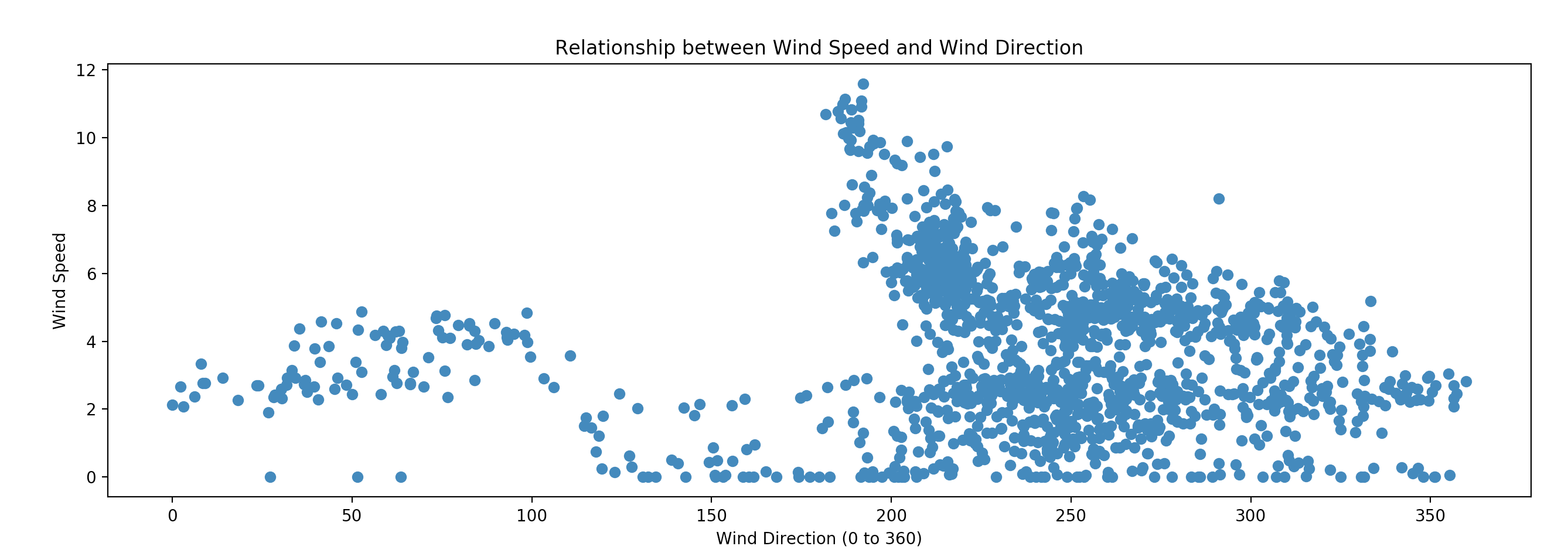
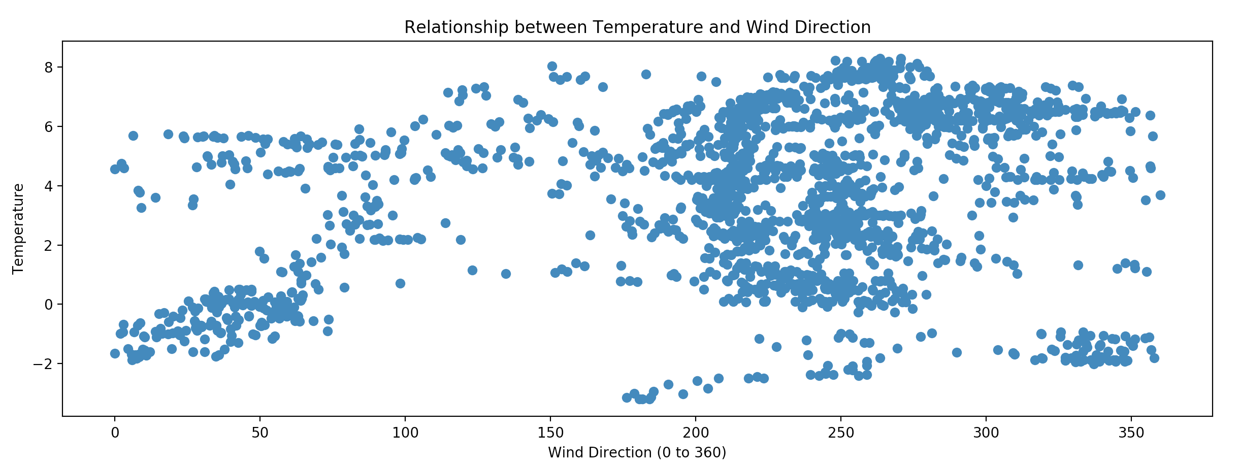
There were two variables in the dataset that I suspected having a relationship with the wind direction: temperature and wind speed.

To determine whether a dependent linear variable and a circular predictor have a relationship, you need to check whether they have a sinusoidal shape. Link

Below are the graphs of wind speed vs wind direction and temperature vs wind direction. You can see they have a loosely sinusoidal shape, which was enough for me to add them to model to see if they added any value in forecasting.

Quadrants

I normalized the temperature and wind speed variables and added them to the circular dataset. Code for adding wind speed and temperature below.

from sklearn.preprocessing import normalize
def setupTrainTestSets(train_test_data,total,recordsBack, trainSet,cos=False):

	i=0
	training_data = []
	wind_direction_actual = []
	wind_speed=[]
	temperature=[]
	actual=[]

	while i <total:
		wind_speed.append(train_test_data.Ws_avg.values[i:recordsBack+i])
		temperature.append(train_test_data.Ot_avg.values[i:recordsBack+i])		
		if(cos):
			training_data.append(train_test_data.cos.values[i:recordsBack+i])
			wind_direction_actual.append(train_test_data.cos.values[recordsBack+i])
		else:
			training_data.append(train_test_data.sin.values[i:recordsBack+i])
			wind_direction_actual.append(train_test_data.sin.values[recordsBack+i])
		
		actual.append(train_test_data['Wa_c_avg'].values[recordsBack+i])
		i+=1

	training_data=np.array(training_data)
	wind_direction_actual=np.array(wind_direction_actual)
	
	wind_speed=np.array(wind_speed)
	wind_speed=normalize(wind_speed)
	
	temperature=np.array(temperature)
	temperature=normalize(temperature)

	
	training_data=np.reshape(training_data, (training_data.shape[0], training_data.shape[1],1))
	wind_speed=np.reshape(wind_speed, (wind_speed.shape[0], wind_speed.shape[1],1))
	temperature=np.reshape(temperature, (temperature.shape[0], temperature.shape[1],1))

	
	training_data=np.concatenate((training_data, wind_speed), axis=2)
	training_data=np.concatenate((training_data, temperature), axis=2)

Model optimization¶

I trained models with combinations of different loss and optimization functions to find the best fitting options.

Loss functions tested:¶

mean_squared_error
mean_absolute_error *Performed better on validation set

Optimization functions tested:¶

RMSprop
Adam *Performed better on validation set

Additionally I tried the following structures in my LSTM models. A single layer with 128 nodes proved best.

Single layer models tried:¶

64 nodes
128 nodes
256 nodes

Two layer models tried:¶

Layer 1: 128 nodes, Layer 2: 64 nodes
Two 64 node layers
Two 64 node layers with dropout=.2 after second layer

Results¶

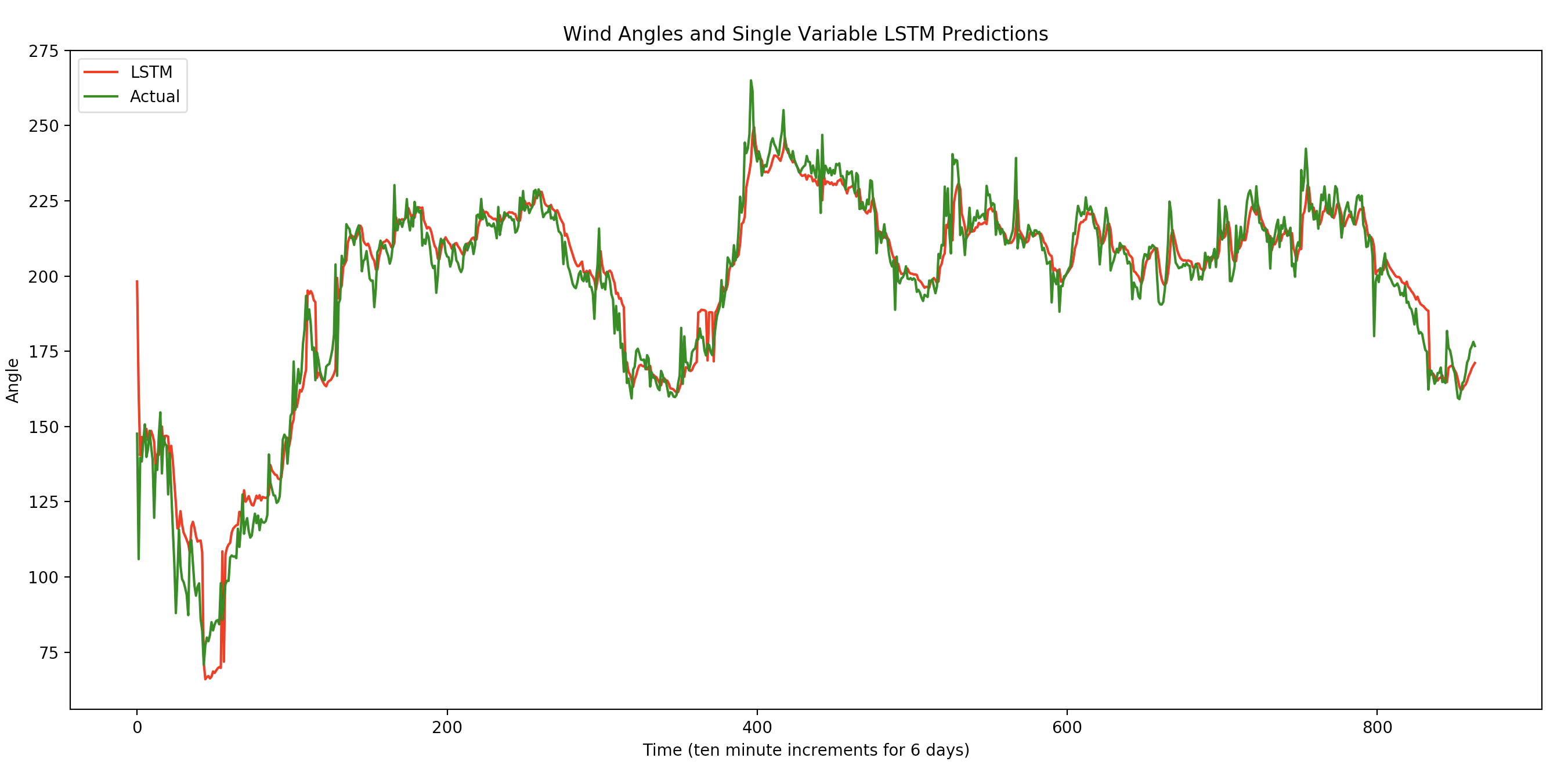
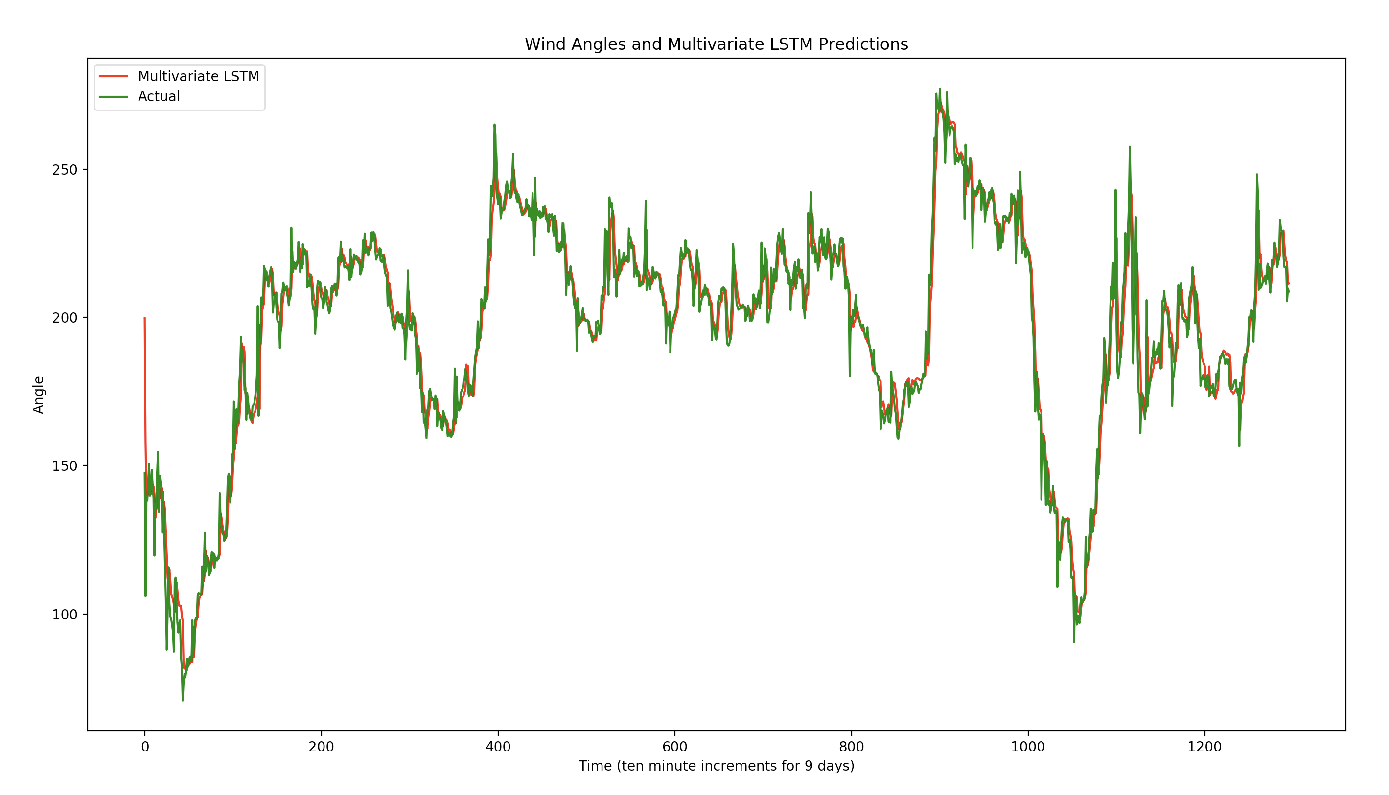
Here are the root mean square error and mean absolute error for the predicted angles for each of the three trained models. Each model gets progressively better.

SVR¶

Date	RMSE	MAE
2016-01-01	23.77	18.78
2016-01-02	22.41	17.44
2016-01-03	17.6	14.13
2016-01-04	12.38	9.31
2016-01-05	8.84	7.21
2016-01-06	7.56	5.79

Single variable LSTM¶

Date	RMSE	MAE
2016-01-01	14.03	10.63
2016-01-02	5.47	4.25
2016-01-03	7.37	5.36
2016-01-04	6.64	4.61
2016-01-05	5.7	4.12
2016-01-06	6.75	4.81

Multivariate LSTM¶

Date	RMSE	MAE
2016-01-01	11.2	7.29
2016-01-02	4.5	3.28
2016-01-03	5.99	4.29
2016-01-04	6.40	4.08
2016-01-05	5.40	3.82
2016-01-06	5.78	4.01
2016-01-07	7.69	5.10
2016-01-08	11.69	8.2
2016-01-09	7.11	4.99

LSTM¶

Quadrants

Multivariate LSTM¶

Quadrants

Between 1/1/2016 and 1/6/2016:
Average MAE single variable LSTM: 5.63
Average MAE multi variable LSTM: 4.46

Average RMSE single variable LSTM: 7.66
Average RMSE multi variable LSTM: 6.54

Notes¶

For both MAE and RMSE the multivariate LSTM performed better
Training on the multivariate LSTM takes longer
Optimization was performed with a smaller training dataset (10 days) because of the length of training. Adding CuDNNLSTM helped, however, training was still very long for each day.
Single and multivariate LSTM are more computationally expensive than SVR
Source code