An RL-like ensembling technique applied to forecasting
While wandering South America at the end of 2018 my mind was consumed with (aside from nature) thoughts of reinforcement learning . I kept wondering how I could apply these technique to some of my recent personal projects with forecasting. Some have tried to apply reinforcement learning to idealized trading games, but time series don't seem to be a very good arena for what RL was meant for.
One rainy day in Bariloche the thought crossed my mind to use RL as an ensembling technique. If I have a bunch of models that are performing guesses on the same data, could I provide them with a reward mechanism so as to choose the right model at each time step?
I constructed an idea in my mind on how to implement such a model when I got back to Ohio. This much thinking without coding was incredibly beneficial to me. I decided I wanted financial data to be the training dataset, since it is classically hard to predict and stochastic in nature. The goal for me was to simply outperform the dreaded persistance model.
My ensemble looks looks very similar to Hinton's Mixtures of Experts model. However my models don't have the variance that would be expected of a Mixtures of Experts model, and so I instead manipulate each models outputs with a function to train the gating network and then randomly sample during online learning.
Ensemble Pruning
Ensembling involves combining two or more models together to produce a better overall performance. A simple way to do this in a regression set would be averaging the two outputs. Other methods include bagging, boosting, and stacking.
Ensemble pruning involves selecting only a subset of the models to prune out of the ensemble to use for prediction. Reinforcement Learning was applied as an ensembling technique for classification data in a 2009 paper, however they did not explore their technique on regression data.
Code: https://github.com/mattgorb/RL_EnsemblePruning
Data Setup
- One-step ahead prediction was performed on the dataset.
- Because of one-step ahead prediction, I need to rescale the data at each time step during test time so that future data doesn't influence training data.
- HAAR tranformation is a simple denoising technique. I use it to even out the curves in a time series graph. PyWavelets make this task super easy. I got the idea from a paper that uses standard techniques for time series forecasting to build stacked autoencoders for better predictions.
- Time Series data is typically scaled between -1 and 1. I used SkLearn for this task.
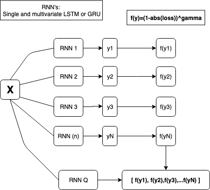
Recurrent Model Stack
Multivariate models do better, so I weigh the stack heavily in favor of them
def model_stack():
    multivariate_models={
        "multi_lstm_512":multivariateLSTM(512,'mse',time_steps_back),
        "multi_lstm_128":multivariateLSTM(1024,'mse',time_steps_back),
        "multi_gru_512":multivariateGRU(512,'mse',time_steps_back),
        "multi_gru_256":multivariateGRU(256,'mse',time_steps_back),
        "multi_gru_2":multivariateGRU(700,'mse',time_steps_back),
        "multi_gru_3":multivariateGRU(400,'mse',time_steps_back),
        "multi_gru_1024":multivariateGRU(1024,'mse',time_steps_back),
        "multi_gru_4":multivariateGRU(300,'mse',time_steps_back),
        "multi_lstm_3":multivariateLSTM(400,'mse',time_steps_back),
        "multi_lstm_4":multivariateLSTM(800,'mse',time_steps_back),
        "multi_lstm_5":multivariateLSTM(1300,'mse',time_steps_back),
        "multi_lstm_6":multivariateLSTM(550,'mse',time_steps_back)
        }
    singlevariate_models={
        "single_GRU_64":singleGRU(64,'mse',time_steps_back),
        "single_GRU_32":singleGRU(128,'mse',time_steps_back)}

    multivariate_models = OrderedDict(sorted(multivariate_models.items(), key=operator.itemgetter(0)))
    singlevariate_models = OrderedDict(sorted(singlevariate_models.items(), key=operator.itemgetter(0)))
    return multivariate_models,singlevariate_models


def multivariateGRU(nodes, loss,time_steps_back):
    model = Sequential()
    model.add(GRU(nodes, input_shape=(time_steps_back,19)))
    model.add(Dense(1))
    model.compile(loss=loss, optimizer='adam')
    return model


def train(model,weights_file,x,y,valX,valY,batch,epochs):
    history = History()
    reduce_lr = ReduceLROnPlateau(monitor='val_loss', factor=0.5, patience=2, min_lr=0.000001, verbose=0)
    checkpointer=ModelCheckpoint('weights/'+weights_file+'.h5', monitor='val_loss', verbose=0, save_best_only=True, save_weights_only=True, mode='auto', period=1)
    earlystopper=EarlyStopping(monitor='val_loss', min_delta=0.0003, patience=5, verbose=0, mode='auto')
    model.fit(x, y, validation_data=(valX, valY),epochs=epochs, batch_size=batch, verbose=0, shuffle=True,callbacks=[checkpointer, history,earlystopper,reduce_lr])
    lowest_val_loss=min(history.history['val_loss'])
    print(lowest_val_loss)
    return model,lowest_val_loss
Ensemble Pruning
The pruning model uses the same techniques as a deep-q network. Each model creates an output, and we convert the output into a reward. I "stretch" the reward by raising to power 20, and the Q output matrix becomes a reward for each model in the stack. I then randomly sample these values during test time, train the Q network, and select the best model to output.
Step-by-step
After training each neural network, I train the ensemble network by performing the following:
- Output the prediction for each training step from each model in the ensemble.
- Calculate the absolute loss: absolute_value(actual[i]-prediction[i])
- Calculate the "reward": 1-absolute_value(loss). Since data is scaled between -1 and 1, this works.
- "Stretch" the values: (1-absolute_value(loss))^gamma.
For me, gamma was 20. My methodology was to take the average validation data loss of each model and calculate gamma for (1-loss)^gamma=0.5. This way the network would retain an even output space across 0-1. - Add this data into the training sample.
- For each new prediction randomly sample training data, similar to a Deep-Q network, and train. From here, make a prediction about the new data.
- Add new data to pool of training data to sample.
Example:
Ensemble consists of two models.
Model 1 prediction=0.97
Model 2 prediction=0.95
Actual value=0.99
Model 1 loss=abs(.97-.99)=0.02, Reward=1-0.02=0.98
Model 2 loss=abs(.95-.99)=.04, Reward=0.96
"Stretched Rewards":
0.98^20=0.667
0.96^20=0.442
Qy=[0.667,0.442]
The Q network will be able to perform much better with these two values than if it were trying to choose between 0.96 and 0.98
def Ensemble_Network(nodes,loss,num_models):
    model = Sequential()
    model.add(GRU(nodes, input_shape=(150,19)))
    model.add(Dense(num_models))
    model.compile(loss=loss, optimizer='adam')
    return model


###Test Time Example
for i in range(1,63):
    idx = np.random.choice(np.arange(len(ensemble_Y)), 20, replace=False) #randomly sample 20 values from training data

    x_sample = ensemble_X[idx]
    y_sample = ensemble_Y[idx]

    ensembleModel.fit(x_sample, y_sample, epochs=5, batch_size=5, verbose=0)

    ensemble_prediction=ensembleModel.predict(testData)
    print(ensemble_prediction)
    best=np.argmax(ensemble_prediction) #choose model with highest reward

    ensemble_X=np.concatenate((ensemble_X, testData)) #add to training data once complete.
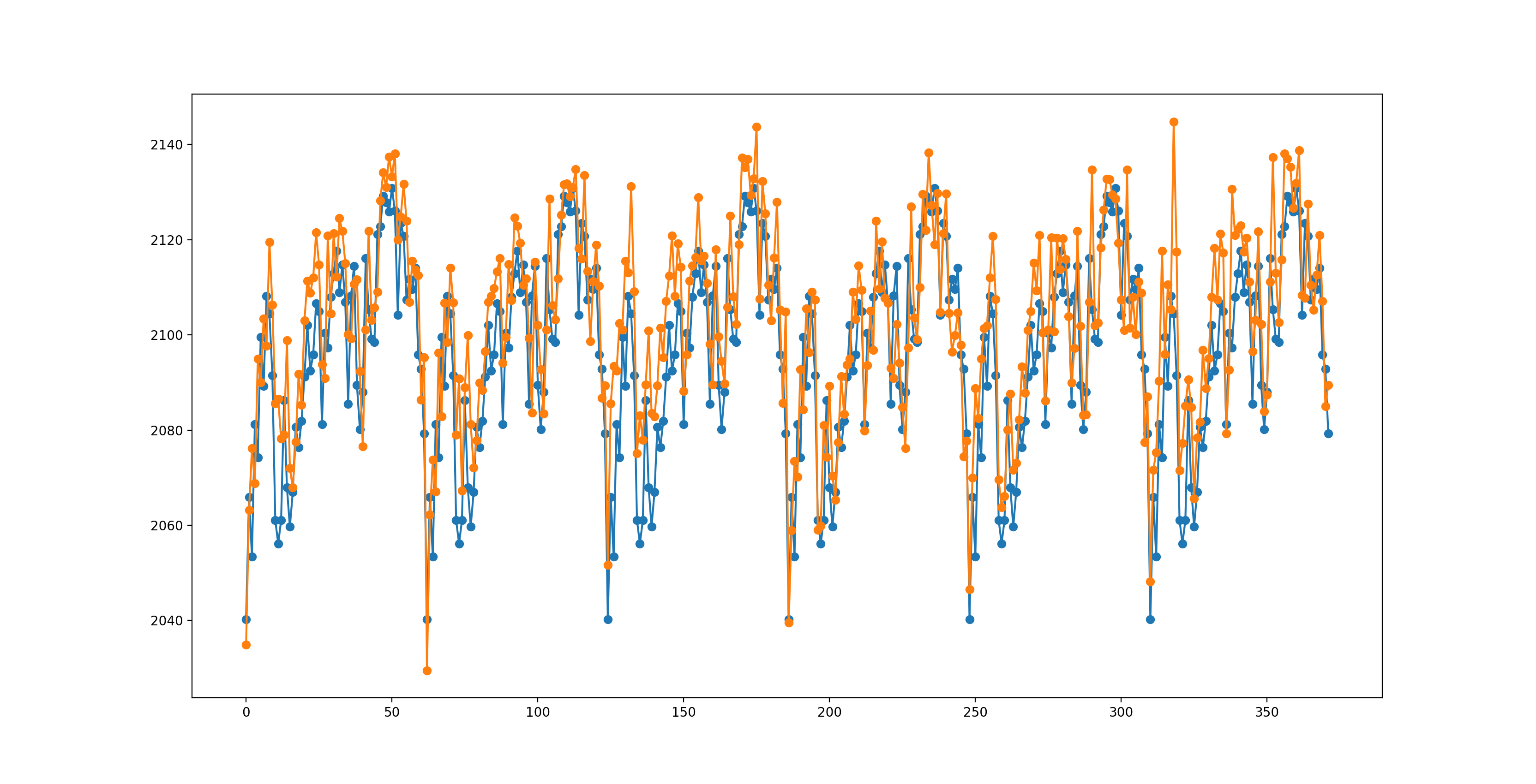
Performance
Ensemble Model: 10.519 MAE
Persistance Model: 11.62533 MAE
Orange is the ensemble, blue are actual values.
Improvements
Currently the code only guesses the best performing model out of all the models and uses that prediction for its final prediction. This was easiest to implement, so I stuck with it. Instead, you could one of the following:
- Pick the top n models from the ensemble networks predictions, take their outputs, and average them.
- Pick models above some threshold i and take their average.