Wind Direction Time Series Forecasting with Support Vector Regression and LSTM Recurrent Neural Network¶

Wind Turbines have dozens of sensors that capture data on various environmental and machine component variables. I came across a public dataset from the company Engie in France that presents data for four wind turbines from 2013-2016. A few variables from the dataset include wind speed, wind direction, and nacelle angle. Source code

The Problem¶

The body of a wind turbine, known as the nacelle, has sensors on it that provide information on the wind speed and wind direction. This information is used for the wind turbine to turn, or "yaw", to face the wind to produce maximum power output. However, the sensors are sometimes faulty and/or not calibrated correctly and give off bad information, causing the turbine to not be in alignment with the direction of the wind. This is known as yaw error. Being able to bring the yaw error closer to zero degrees would increase the power output of the wind turbine. This could be done by implementing a prediction algorithm into a yawing controller.

I'll be exploring whether wind direction can be predicted accurately based on historical data. I'll be using the following tech stack to try and solve this as a time series machine learning problem:

Python 3.6: Pandas, NumPy
Sklearn
Keras (TensorFlow API)
Matplotlib

A brief look at yaw error¶

Below I look at data for a single wind turbine in 2016 and find the difference between the wind direction angle (Wa_C_avg) and the nacelle yaw angle (Ya_avg). After taking the absolute value of the differences, you can see that the yaw error is on average 13.55 degrees, which is pretty high.

import pandas as pd
import numpy as np
import datetime

df = pd.read_csv('la-haute-borne-data-2013-2016.csv', sep=';')
df['Date_time'] = df['Date_time'].astype(str).str[:-6] #remove timezone
df.Date_time=pd.to_datetime(df['Date_time'])
df=df.fillna(method='ffill')
df=df[df['Wind_turbine_name']==df.Wind_turbine_name.unique()[0]] 
df=df.sort_values(by='Date_time')
turbineOne_2016=df[df['Date_time']>= datetime.datetime(2016, 1, 1)]

diff=np.abs(turbineOne_2016.Wa_c_avg.values-turbineOne_2016.Ya_avg.values)
diff=diff[np.where(diff<300)] #Since the data is in circular angles (0-360), filtering out differences>300
print("Length of Dataset")
print(len(diff))
print("Number with yaw error")
print(np.count_nonzero(np.abs(diff)))
print("Average yaw error")
print(np.mean(diff))

Length of Dataset
51977
Number with yaw error
51956
Average yaw error
13.55402167992462

Data¶

The data in the La Haute-Borne dataset is logged every 10 minutes, for each day there are 6*24=144 predictions. The model I built uses a day as a test set, with the training set being the previous 90 days.

Transforming angles into usable variables¶

Wind direction is a circular variable, meaning the output is given in degrees between 0 and 360. To transform this variable into data usable for circular regression, I'll use the following equation:

y^=β1cos(π∗angle/360)+β2sin(π∗angle/360)¶

With NumPy and Pandas, its easy to execute these functions:

df['sin']=np.sin(df['Wa_c_avg']/360*2*math.pi)
df['cos']=np.cos(df['Wa_c_avg']/360*2*math.pi)

Transforming sine and cosine into prediction angle¶

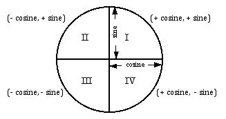
To transform sine and cosine predictions back into actual angle predictions, it depends on the value of both sine and cosine. The image below shows the quadrant the prediction will fall into given the predicted sine and cosine values. For example, if both sine and cosine are less than zero, the predicted angle will fall between 180 and 270 degrees.

Quadrants

The below functions are helper functions for converting predictions back into a single angle prediction. I use RMSE, Root Mean Squared Error, to find the error of both the sine and cosine models. I weight the model in favor of the lowest error model. For example, if the sine model has an error of 0.05, and the cosine error is .1, I weight the sine model with 2/3 and the cosine model with 1/3.

def convertToDegrees(sin_prediction,cos_prediction):
	'''
	Converting sine and cosine back to its circular angle depends on finding which of the the 4 circular quadrants the 
	prediction will fall into. If sin and cos are both GT 0, degrees will fall in 0-90.  If sin>0 cos<0, degrees will fall into 90-180, etc. 
	'''
	inverseSin=np.degrees(np.arcsin(sin_prediction))
	inverseCos=np.degrees(np.arccos(cos_prediction))
	radians_sin=[]
	radians_cos=[]
	for a,b,c,d in zip(sin_prediction, cos_prediction, inverseSin, inverseCos):
		if(a>0 and b>0):
			radians_sin.append(c)
			radians_cos.append(d)	
		elif(a>0 and b<0):
			radians_sin.append(180-c)
			radians_cos.append(d)	
		elif(a<0 and b<0):
			radians_sin.append(180-c)
			radians_cos.append(360-d)	
		elif(a<0 and b>0):
			radians_sin.append(360+c)
			radians_cos.append(360-d)
	radians_sin=np.array(radians_sin)
	radians_cos=np.array(radians_cos)
	return radians_sin, radians_cos

Support Vector Regression Training¶

To build a dataset, Support Vector Regression requires building data into the following structure:

x1	x2	x4	x4	x5	y
y(t-5)	y(t-4)	y(t-3)	y(t-2)	y(t-1)	y(t)

That is, for predicting a value y(t), you must send it y(t-n), y(t-(n-1))...y(t-1) as input values.

I built the models using only their historic sine and cosine values, respectively. I used sklearn.SVM's SVR library for regression.

C and Gamma were tuned depending on the size of the dataset. I found that for a bigger dataset, bigger C and smaller gamma did well. These were tuned over many runs on different days to find the best values.

Below is the train and predict function, which creates a feature array (x) and prediction array (y) in numpy. X and y are trained on values up to the length of the dataset minus 144. The remaining 144 inputs/outputs are used as the test set.

from sklearn.svm import SVR

def train_predict(train_test_data, c_,g_, cos=False):
	i=0
	x = []
	y = []
	while i <total:
		if(cos):

			x.append(train_test_data.cos.values[i:recordsBack+i])
			y.append(train_test_data.cos.values[recordsBack+i])
		else:
			x.append(train_test_data.sin.values[i:recordsBack+i])
			y.append(train_test_data.sin.values[recordsBack+i])
		i+=1

	svr_rbf = SVR(kernel='rbf', C=c_ ,gamma=g_)
	y_rbf = svr_rbf.fit(x[:trainSet], y[:trainSet]).predict(x)
	y_rbf[y_rbf > 1] = 1
	y_rbf[y_rbf < -1] = -1
	mae = mean_absolute_error(y[trainSet:], y_rbf[trainSet:])
	mse = mean_squared_error(y[trainSet:], y_rbf[trainSet:])
	rmse = sqrt(mse)

	return y_rbf[trainSet:], rmse

Sine/Cosine Ensemble Model¶

The method calcWeightedRMSEDegreePredictions below combines the sine and cosine models into a single prediction using the values of each train sets RMSE. For example, if model 1 has RMSE=5 and model 2 has RMSE=10, the weights for each prediction will be:

Model 1=(15-5)/15=2/3
Model 2=(15-10/15=1/3

We want to apply more weight to the model that appears to have higher accuracy, so we weight them by how close they are to an error of zero.

def calcWeightedRMSEDegreePredictions(sin_rmse,cos_rmse,radians_sin,radians_cos):
	rmseTotal=cos_rmse+sin_rmse
	sinWeight=(rmseTotal-sin_rmse)/rmseTotal
	cosWeight=(rmseTotal-cos_rmse)/rmseTotal
	weighted=np.add(sinWeight*radians_sin, cosWeight*radians_cos)
	return weighted

SVR Test Results¶

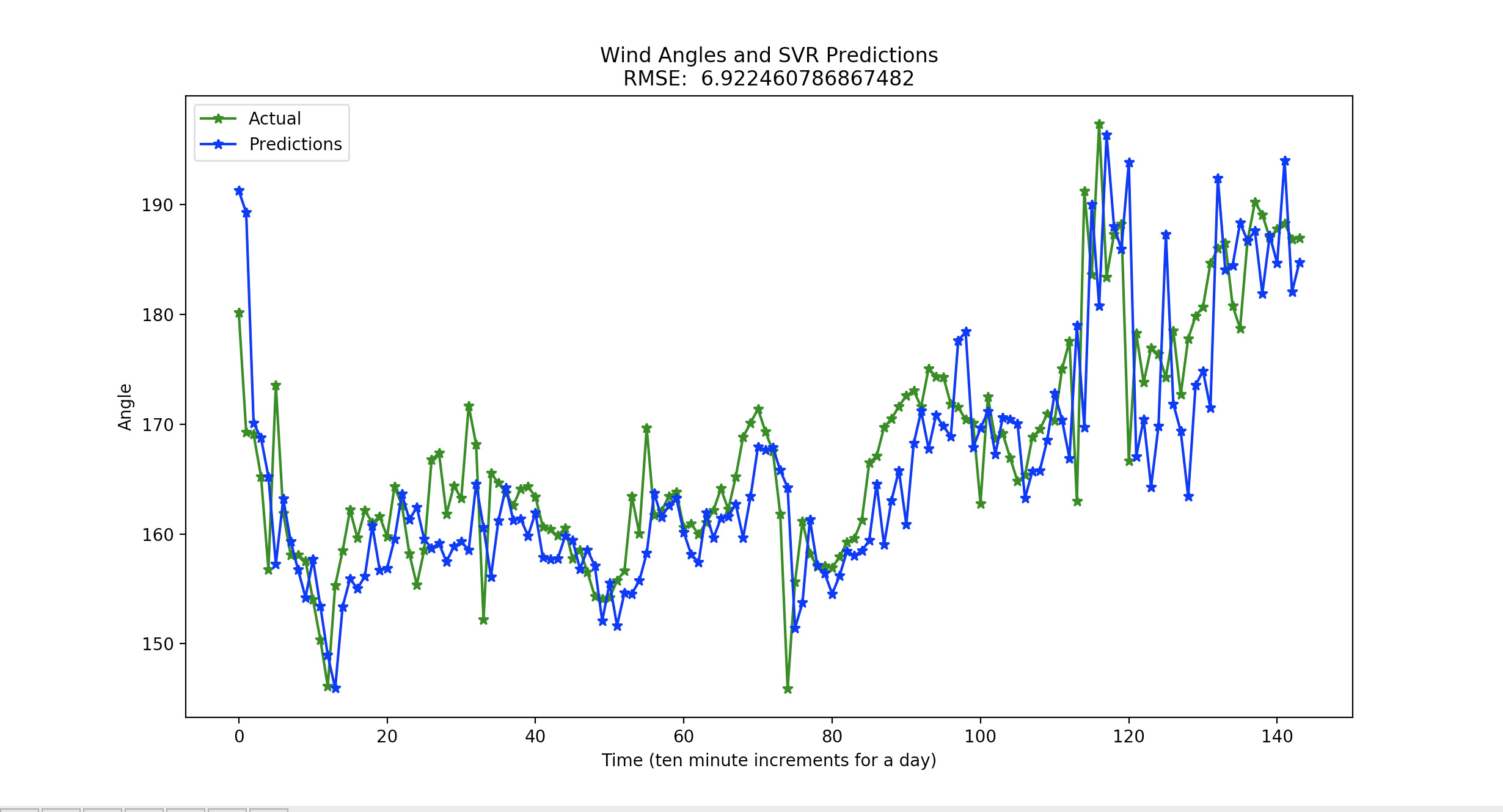
The root mean squared on any random day is between about 6 and 10. The following is an example output with a root mean squared error of 6.92246 degrees.

TimeSeries

A note on SVR complexity¶

SVM-training with nonlinear-kernels, which is default in sklearn's SVC, is complexity-wise approximately: O(n_samples^2 * n_features)

StackOverflow post

I found that the more history I tried to add into the dataset, the longer my training would take. I limited my training to 90 days back by 6 days back. Some variables set in my SVR training:

previousDays_rows=90
trainSet=previousDays_rowsx24x6 #train on 90 previous days of data
previousDays_columns=6
recordsBack=previousDays_columnsx24x6

This meant the datasets I sent to the model had a shape (90246, 6246)=(12960,864).

Long Short Term Recurrent Neural Network¶

Data¶

For the LSTM network I again trained sine and cosine models. I'll be using four different datasets:

Partial training dataset
Validation dataset
Full training dataset
Test dataset

First I will train a model with a validation set equal to the test day minus one day. I will use the validation error to compute weights in the neural network and save off the best iteration of this model. My theory here is to train a model that will generalize predictions on data that the model hasn't seen, the validation set. Once the model has found ideal weights for this unseen data, I will train it on another iteration of the model with the full amount of data. This full amount of data is important to the model because the most recent data is significant when predicting time series. To give an example:

I want to predict the wind directions on for January 2, 2016. To do this, take the last year of wind directions and split them up like so: 1/2/2015-12/31/2015-Partial training dataset
1/1/2016-Validation dataset 1/2/2015-1/1/2016-Full training dataset 1/2/2016-Test set
The method below does the following:

Push the partial training dataset into the neural network. The neural network will train this dataset. To test, it will use the validation dataset. It saves neuron weights based off of which weight combinations have the smallest error on the validation set.
Once the ideal weights are found for the trained model, I will load the full training dataset into the model and train for one more iteration. This models weights update to take into account the extra day of data.
I can then use the model and its weight to predict the output for January 2nd.

Below is the method for breaking up data into its corresponding arrays:

def setupTrainTestSets(train_test_data,total,recordsBack, trainSet,cos=False):
	i=0
	x = []
	y = []
	actual=[]
	while i <total:
		if(cos):

			x.append(train_test_data.cos.values[i:recordsBack+i])
			y.append(train_test_data.cos.values[recordsBack+i])
			
		else:
			x.append(train_test_data.sin.values[i:recordsBack+i])
			y.append(train_test_data.sin.values[recordsBack+i])
		
		actual.append(train_test_data['Wa_c_avg'].values[recordsBack+i])
		i+=1

	x=np.array(x)
	y=np.array(y)

	trainX_initial=x[:trainSet-144]
	trainY_initial=y[:trainSet-144]

	validationX=x[trainSet-144:trainSet]
	validationY=y[trainSet-144:trainSet]

	trainX_full=x[:trainSet]
	trainY_full=y[:trainSet]

	testX=x[trainSet:]
	testY=y[trainSet:]
	actual=np.array(actual[trainSet:])

	testX = np.reshape(testX, (testX.shape[0], testX.shape[1],1))
	trainX_initial=np.reshape(trainX_initial, (trainX_initial.shape[0], trainX_initial.shape[1],1))
	trainX_full=np.reshape(trainX_full, (trainX_full.shape[0], trainX_full.shape[1],1))
	validationX=np.reshape(validationX, (validationX.shape[0], validationX.shape[1],1))
	return trainX_initial, trainY_initial, validationX, validationY, trainX_full, trainY_full, testX,testY, actual

Training¶

For Keras model training, I decided to use mean absolute (MAE) as the error function. I tuned the network to only include a single hidden layer with 128 nodes. Additionally, I input the numpy array with dimensions=(rows, columns (time periods), features=1)

I included two callbacks in the the model fit, ModelCheckpoint and EarlyStopping:

ModelCheckpoint monitors val_loss, which is the validation dataset error, and saves the lowest validation dataset error to a file named weights.h5. It writes weights to the file whenever the val_loss improves.

EarlyStopping monitors the validation error and stops the training if the validation error hasn't improved in 3 iterations (patience parameter). Since neural networks take a long time to train, especially on a CPU, this helps with training time.

If predictions fall outside of the range [-1,1], I round them up or down, since sine and cosine values can't fall outside this range.

Sine and cosine models were combined the same way as the SVR method above, using the error function to weight each model for a final prediction.

from keras.callbacks import EarlyStopping, ReduceLROnPlateau, ModelCheckpoint, TensorBoard
from keras.models import Sequential
from keras.layers import Dense
from keras.layers import LSTM

def train_predict():
        model = Sequential()
        model.add(LSTM(128, input_shape=(recordsBack,1)))
        model.add(Dense(1))
        model.compile(loss='mean_absolute_error', optimizer='adam')


        checkpointer=ModelCheckpoint('weights.h5', monitor='val_loss', verbose=2, save_best_only=True, save_weights_only=True, mode='auto', period=1)
        earlystopper=EarlyStopping(monitor='val_loss', min_delta=0, patience=3, verbose=0, mode='auto')
        model.fit(trainX_initial, trainY_initial, validation_data=(validationX, validationY),epochs=50, batch_size=testX.shape[0], verbose=2, shuffle=False,callbacks=[checkpointer, earlystopper])

        model.load_weights("weights.h5")

        validationPredict=model.predict(validationX)
        validation_mae=mean_absolute_error(validationY, validationPredict)

        model.fit(trainX_full, trainY_full, epochs=1, batch_size=testX.shape[0], verbose=2, shuffle=False)
        testPredict = model.predict(testX)

        testPredict[testPredict > 1] = 1
        testPredict[testPredict <-1] = -1
        return testPredict, validation_mae

LSTM Test Results¶

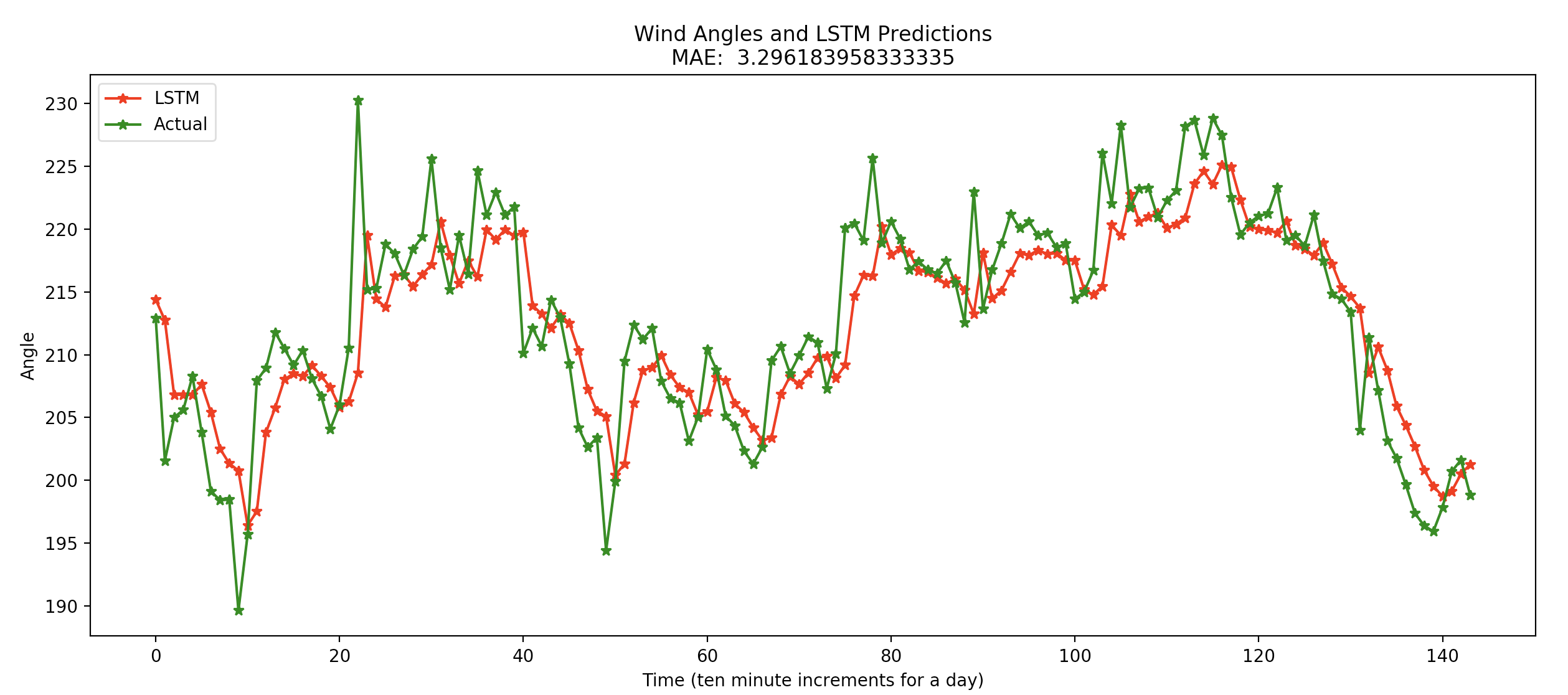
Results for January 2nd, 2016

TimeSeries

Conclusion¶

LSTM networks performed better overall on most test sets. Limitations in SVR computation accentuate LSTM's superiority for this data. I was able to train LSTM models on significantly larger datasets using only CPU computation.

Possible Enhancements¶

Explore multivariate LSTM networks. Dozens of variables from wind turbine sensor data are available in the dataset I used and making use of variables such as wind speed and temperature could potentially improve results.
Run TensorFlow GPU for quicker LSTM Training. Training time would be vital in any real-world implementation of wind directon prediction as time series need up to date training datasets for better accuracy
Explore further ensemble modeling.
Train LSTM on larger dataset.
Explore different model structures in LSTM network.
Explore different loss and optimization functions.