Artificial Neural Network
The following code is a simple three layer neural network written in Python and NumPy. This was my first shot at programming a neural network, so there may be some issues with it. I wanted to build it from scratch so I could attempt to understand and conceptualize the math involved.
A neural network is a learning algorithm that attempts to solve complex problems in computer vision, speech recognition, and other fields in artificial intelligence. Artificial Neural Networks were named after their similarity to the human brain, with its millions of neurons and axons receiving inputs from the external environment and creating electrical impulses which travel through the connected network of the brain.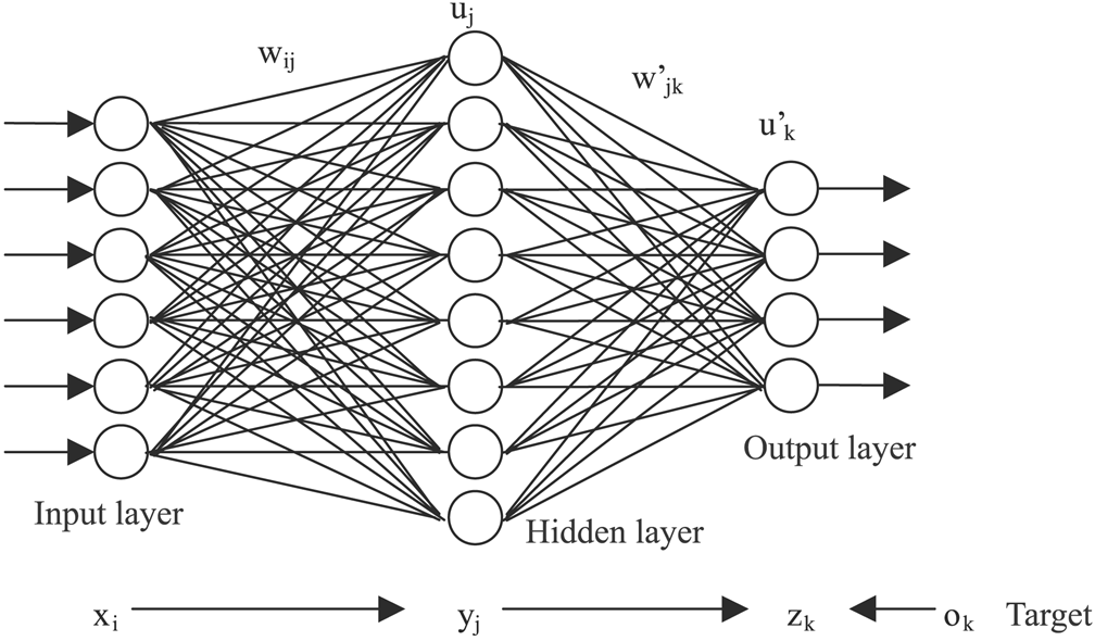
Data
I'm going to be using NumPy here, which is a linear algebra library for Python. I read all my data from csv. A basic function of this is below which creates two matrices, inputData and outputData. The output data is in the fifth column of the csv file and the input data is from the sixth column to the last column.
#Basic, stripped down data load from a CSV file to two NumPy arrays
def LoadData(fileName, start,end):
    inputData=[] #python array
    outputData=[]
    with open(fileName, 'rb') as csvfile:
        reader = csv.reader(csvfile, delimiter=',')
        for row in itertools.islice(reader, start,end): #itertools is a python iterator tool
            output=np.longfloat(row[5]) #output is the fifth index in each row
	    #create a numpy long float array for each row from the sixth index to the last (len(row)) index
            input = [np.longfloat(x) for x in itertools.islice(row , 6,len(row) ) if x != '']
	    #add each row to the python array
            inputData.append(input)
            outputData.append(output)
    return inputData,outputData
Note that the input data should already be normalized. I'm not going to talk about this, but it is a very important piece to building a working neural network.
Links on data normalization: Data Normalization in Neural Networks How to Standardize data for Neural Networks
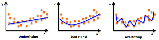
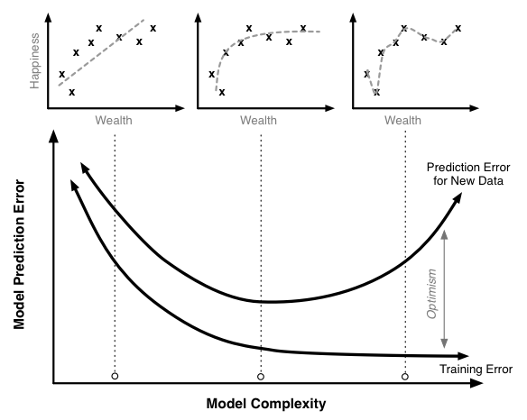
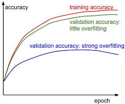
Another important facet of supervised learning is the three different types of datasets. I'll go over these below.
Stats and graphs and stuffs
Training in python, NumPy
def Train(self):
    global weights0,weights1,layer1_deltaPrev,layer2_deltaPrev

    #training iterations are set by the user in the program initialization.
    for iter in xrange(self.trainingIterations):

   	#layer 0 equals the training inputs in NumPy matrix form.
        layer0 = self.TrainingIn

        #neural nets should always use shuffle.  One big bug in this program is that the outputs are in a separate
        #matrix.  This means that randomly shuffling the inputs is going to give them random outputs.  For my training
        #I set shuffle to off.
        if(self.shuffle):
	    np.random.shuffle(layer0)

	#np.dot is a NumPy multiplication function.  It multiplies layer0(input) by the randomly initialized weights, and is fed through the sigmoid function self.nonlin
        layer1 = self.nonlin(np.dot(layer0,self.weights0))

	#you should always include a bias layer. This means adding a column of 1's to your matrix
        if(self.biasLayer1TF):
            self.biaslayer1 = np.ones(layer1.shape[0])
            layer1=np.column_stack((layer1,self.biaslayer1))

        #dropout should also always be used.  0>dropout<1
        if(self.dropout):
            layer1 *= np.random.binomial([np.ones((layer1.shape[0],layer1.shape[1]))],1-self.dropoutPercent)[0]

        #layer2 equals layer1*weights1 fed through the sigmoid function self.nonlin
        #layer2 is what the network is predicting the output will be.
        layer2 = self.nonlin(np.dot(layer1,self.weights1))

        #more on this later
        if(self.miniBtch_StochastGradTrain):
            self.layer1_delta,self.layer2_delta=self.MiniBatchOrStochasticGradientDescent()
            self.layer2_deltaPrev=self.layer2_delta
            self.layer1_deltaPrev=self.layer1_delta
        else:

	    #the error= the distance between the guesses from the actual values.
            layer2_error = self.TrainingOut - layer2

            #take the derivative (slope) of each node in layer2, and multiply it by the error.  The higher the error,
            #the more the slope delta will be.  Learning rate is also applied here, which is how fast you want your network to correct
            #itself.  Additionally momentum is applied to the end of this, which is added the previous iterations deltas to the current iteration
            self.layer2_delta = layer2_error*self.nonlin(layer2,deriv=True)*self.learningRate+self.momentum*self.layer2_deltaPrev
            self.layer2_deltaPrev=self.layer2_delta

	    #.T means the transposed matrix in Numpy.
            layer1_error = self.layer2_delta.dot(self.weights1.T)
            self.layer1_delta = layer1_error * self.nonlin(layer1,deriv=True)*self.learningRate+self.momentum*self.layer1_deltaPrev
            self.layer1_deltaPrev=self.layer1_delta

	#update the weights in each layer with the delta layers
        self.weights1 += layer1.T.dot(self.layer2_delta)
        if(self.biasLayer1TF):
            self.weights0 += layer0.T.dot(self.layer1_delta.T[:-1].T)
        else:
            self.weights0 += layer0.T.dot(self.layer1_delta)


        if (iter% 20) == 0:
            self.CalculateValidationError()

            if(self.minimumValidationError<0.01):
                break
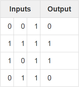
Looking at the table we have 4 rows with 3 variables of input data. The output data is 4 rows with 1 result. So we will have a TrainIn matrix of size 4x3 and a TrainOut matrix of 4x1. The above table looks like the following in a NumPy array: TestIn = np.array([ [0,0,1],[0,1,1],[1,0,1],[1,1,1] ]) TestOut = np.array([[0,1,1,0]]).T Note the ".T" in the TestOut variable. This means transpose the matrix. It is visualized here as a 1x4 matrix, by transposing it we create a 4X1 matrix, conducive to our input set.
Since we are working with such a simple dataset I'm going to skip over validation data and test data. Our test data will simply be our training data.Now that we have input data to send to the network, I'm going set the parameters for the network. I do this in main.py. These parameters get sent to the Neural Network class and initialize the model. I'm going to concentrate on the parameters hiddenDim, learningRate, trainingIterations, momentum, and dropout. Below is the parameter dictionary I send to the Neural Network class.
Run({"hiddenDim":2,"learningRate":.05,"trainingIterations":5000,"momentum":.1,
"dropout":True,"dropoutPercent":0.65,
 "miniBtch_StochastGradTrain":"False","miniBtch_StochastGradTrain_Split":null,"NFoldCrossValidation":False,"N":null#skip these,
 "biasLayer1TF":True,"addInputBias":False,"shuffle":False
})
Initializing weights and deltas
np.random.seed(1)
self.weights0 = (2*np.random.random((self.TrainingIn.shape[1],self.hiddenDim)) - 1)
self.weights1 = (2*np.random.random((self.hiddenDim+1 if self.biasLayer1TF else self.hiddenDim,1)) - 1)
np.random.random creates a matrix of random numbers between 0 and 1. It is best practice to initialize the weights randomly with mean 0, so I multiply these numbers by 2 and subtract 1. self.TrainingIn.shape returns the size of the matrix, in our case 4x3. Therefore self.TrainingIn.shape[1] returns the second number of this value, 3. hiddenDim was set to 2 in our initalization parameters above. So self.weights0 will be a matrix of size 3X2 with random numbers between -1 and 1. Since bias is turned off for this example, weights1 will be initialized with a matrix size 2(hiddenDim)x1 with random numbers between -1 and 1. We also need to intialize "layerx_deltaPrev" matrices for momentum. np.zeros creates a matrix of 0's.
self.layer2_deltaPrev=np.zeros(shape=(self.TrainingOut.shape[0],self.weights1.shape[1]))
self.layer1_deltaPrev=np.zeros(shape=(self.TrainingIn.shape[0],self.hiddenDim+1 if self.biasLayer1TF else self.hiddenDim))
Train()
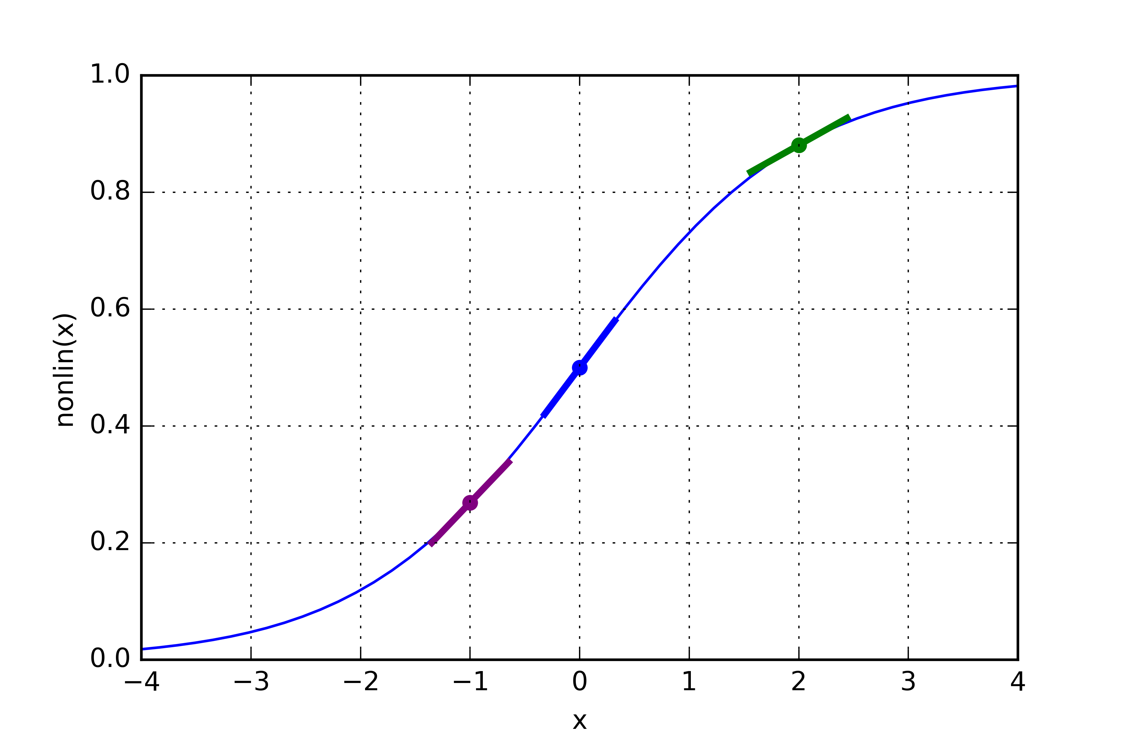
We're ready to enter the Train() method from above. We will iterate in the for loop 5000 times to update the weights of the network based on the input data and expected output. layer0 = self.TrainingIn. Self explanatory. Shuffle is rearranging the data into random rows. The next line of code is doing a lot:layer1 = self.nonlin(np.dot(layer0,self.weights0)def nonlin(self,x,deriv=False):
if(deriv==True):
return x*(1-x)
return 1/(1+np.exp(-x))
Dropout
layer1 *= np.random.binomial([np.ones((layer1.shape[0],layer1.shape[1]))],1-self.dropoutPercent)[0]
layer2 = self.nonlin(np.dot(layer1,self.weights1))
Backpropagation
layer2_error = self.TrainingOut - layer2
self.layer2_delta = layer2_error*self.nonlin(layer2,deriv=True)*self.learningRate+self.momentum*self.layer2_deltaPrev
Momentum
Momentum is the second part of the code in the line above:self.momentum*self.layer2_deltaPrev
self.layer2_deltaPrev=self.layer2_delta
Layer1 error and delta
Calculate layer1_error:layer1_error = self.layer2_delta.dot(self.weights1.T)
self.layer1_delta = layer1_error * self.nonlin(layer1,deriv=True)*self.learningRate+self.momentum*self.layer1_deltaPrev
self.layer1_deltaPrev=self.layer1_delta
Weight updates
This is where the network "learns". We update the weights of the network to more resemble the output data:self.weights1 += layer1.T.dot(self.layer2_delta)